analyzing the october primary debate, using tidytext

what we’ll do in this post

I’m aiming for 3 things:

1. Basic vocabulary around text analysis, as related to tidytext functions
2. Demonstrate tokenization and pre-processing of text
3. Describe some textual data

For this exercise, I’ve pulled down the transcript of the October democratic party primary debate from 10/15/2019. I wanted to work with something fresh, and for this post we can imagine ourselves as a data journalist looking to describe patterns of speech from the different candidates.

fundamental units of text: tokens

Our first piece of vocabulary: “token”. A token is a meaningful sequence of characters, such as a word, phrase, or sentence. One of the main tasks of mining text-data is converting strings of characters into the types of tokens needed for analysis; this process is called tokenization. As far as how this is accomplished with tidytext, the workflow is to create a table (data.frame/tibble) with a single token per row. We accomplish this step using the unnest_tokens() function.

library(tidyverse)
library(tidytext)
library(scico)

# load the debate transcript data
wp <- read_rds("../../static/post/20191017-tidytext-overview/data/20191110-oct-dem-debate-cleaned.rds")

# Cooper's introduction to the debate
wp[[2, 3]] %>% str_sub(1, 128)

## [1] "And live from Otterbein University, just north of Columbus, Ohio, this is the CNN-New York Times Democratic presidential debate."

dd_uni <- unnest_tokens(
 tbl         = wp,
 output      = word,
 input       = txt,
 token       = "words",  # (default) tokenize strings to words
 to_lower    = TRUE,     # (default) set the resulting column to lowercase
 strip_punct = TRUE      # (default) scrub the punctuation from each word
)

# the same line, tokenized into single words (unigrams)
filter(dd_uni, index == 1)

## # A tibble: 112 x 3
##    speaker index word      
##    <chr>   <int> <chr>     
##  1 Cooper      1 and       
##  2 Cooper      1 live      
##  3 Cooper      1 from      
##  4 Cooper      1 otterbein 
##  5 Cooper      1 university
##  6 Cooper      1 just      
##  7 Cooper      1 north     
##  8 Cooper      1 of        
##  9 Cooper      1 columbus  
## 10 Cooper      1 ohio      
## # … with 102 more rows

So, from an initial data frame, we’ve gone from a single row per string to rows for each resulting token. The unnest_tokens() function is key to much of what you’ll do with tidytext, so getting familiar with it is important. Now, because each word is now a row of text, we can start to use existing functions from to do some basic analysis. What if we wanted to track the mentions of terms related to a given topic, like healthcare? Here we’ll create a vector of words, and use cumsum() to track running totals within each speaker.

hc_terms <- c(
  "health", "premium", "premiums",
  "medicare", "sick", "prescription",
  "insurance", "doctor", "medicare", "obamacare"
)

# looking at the top 3 candidates
dd_uni %>%
  filter(speaker %in% c("Biden", "Warren", "Sanders")) %>%
  group_by(speaker) %>%
  mutate(hc = cumsum(word %in% hc_terms)) %>%
  ggplot(aes(x = index, y = hc, color = speaker)) +
  geom_step(size = 1.05) +
  scale_color_scico_d(name = "", palette = "nuuk", direction = -1) +
  labs(
    x = "Remark (debate progress)",
    y = "Mentions",
    title = 'Cumulative mentions of "health", "premium(s)", "medicare",\n"sick", "prescription", "insurance", "doctor",\n"medicare", or "Obamacare"'
  )

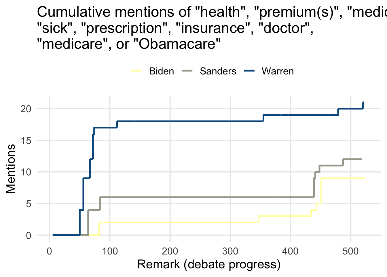
Here you can see Sanders and Warren responding to questions about their policies/plans during the beginning of the debate, and when Sanders and Biden revisit the topic of the insurance industry near the end.

But, you’re definitely not restricted to using just single words! Maybe we want to look for important phrases important to the debate, like “Medicare For All”. A phrase like “Medicare For All” can be thought of as what’s called an n-gram, specifically a trigram. N-grams are just a sequence of n items from a sample of text or speech; in our case our unit/item is words.

We can use unnest_tokens() to pull out all the different trigrams found in our text, and (because the function returns a tidy data frame!) we can then use dplyr::count() to see how many times a given trigram is mentioned.

dd_tri <- unnest_tokens(wp, trigram, txt, token = "ngrams", n = 3)

# count the prevalence of all trigrams found
count(dd_tri, trigram, sort = TRUE) %>%
  slice(1:15)

## # A tibble: 15 x 2
##    trigram                 n
##    <chr>               <int>
##  1 thank you senator      59
##  2 <NA>                   43
##  3 we have to             42
##  4 the united states      37
##  5 we need to             35
##  6 in this country        33
##  7 i want to              31
##  8 we're going to         31
##  9 make sure that         26
## 10 the american people    26
## 11 on this stage          25
## 12 one of the             21
## 13 are going to           19
## 14 medicare for all       18
## 15 thank you mr           18

From this little exercise, it looks like a transitional phrase, “Thank you Senator” (used mostly by the moderators), is the most frequent trigram. However, something worth noting is that the next most common instance is NA– what’s going on here? These simply represent comments that had fewer than 3 words. This is something that we’ll see given that we’re looking at transcribed speech (as opposed to written responses), so it’s important to think about idiosyncracies you might encounter depending on the data you’re analyzing.

handling non-informative words or tokens

In many analyses, it might be important to discard words that aren’t useful or helpful to descrbing the data you’re working with. In natural language processing, these terms/words are referred to as stop words, and they’re generally the most common words found in a language. In the English language, some common stop words include “I”, “is”, “of”, “are”, and “the”. There isn’t a universally accepted list of words that should be discarded, and it’s frequently necessary to augment an existing list with entries that are specific to a given project. For example, we could think about removing the word “senator”, given that many of the debate participants are senators and its usage would be similar to how an honorific like “Mr.” or “Mrs./Ms.” might be used throughout the debate. The tidytext package helpfully includes several lists of stop words, which are a useful starting place for this task. The helper function get_stopwords() enables you to select from a set of 3 lexicons, and supports Spanish, German, and French (in addition to English).

smart_stops <- get_stopwords(language = "en", source = "smart")

head(smart_stops)

## # A tibble: 6 x 2
##   word      lexicon
##   <chr>     <chr>  
## 1 a         smart  
## 2 a's       smart  
## 3 able      smart  
## 4 about     smart  
## 5 above     smart  
## 6 according smart

# here's Cooper's introduction again
# this time we'll drop unigrams that match terms from our list of stop words
dd_uni %>%
  anti_join(smart_stops, by = "word") %>%
  filter(index == 1)

## # A tibble: 65 x 3
##    speaker index word      
##    <chr>   <int> <chr>     
##  1 Cooper      1 live      
##  2 Cooper      1 otterbein 
##  3 Cooper      1 university
##  4 Cooper      1 north     
##  5 Cooper      1 columbus  
##  6 Cooper      1 ohio      
##  7 Cooper      1 cnn       
##  8 Cooper      1 york      
##  9 Cooper      1 times     
## 10 Cooper      1 democratic
## # … with 55 more rows

Note that because each unigram is stored as a row in the data frame, and each stop word is stored as a row in its own data frame, we’re able to discard the ones we don’t want by using dplyr::anti_join().

pulling everything together: using term frequencies and document frequencies

Next we’ll pull each of these preceding steps together to try and identify distinctive words from some of the leading candidates. One common approach to doing this is by generating TF/IDF scores of given terms. TF/IDF is a combination of term frequency and (inverse) document frequency.

Term frequency is merely the fraction of times that a term (in this case, word) appears in a given document.

\(tf(t,d) = \frac{f_{t,d}}{\sum\limits_{t'\in d} f_{t',d}}\)

Document frequency is the number of times a term appears across all documents in a collection. In this case, the measure is inverted so that terms that appear in a small number of documents receive a larger value.

\(idf(t,D) = log\frac{N}{1 + |d \in D : t \in d|}\)

Lastly, the two measures are combined as a product; terms that are found frequently in a small number of documents get higher scores, whereas terms that are found in virtually every document receive lower scores.

\(tfidf(t,d,D) = tf(t, d) \cdot idf(t, D)\)

Calculating each of these metrics is straightforward using the bind_tf_idf() function. bind_tf_idf() simply needs a document ID, a term label, and a count for each term; the results are added to the source data.frame/tibble as new columns. In this case we’ll be treating all the text from each speaker in the debate as a document (thus IDF will be high if every speaker uses a given term).

# create unigrams, drop stop words, calculate metrics
# then, keep each speaker's top 10 terms
top_10_tfidf <- wp %>%
  unnest_tokens(word, txt) %>%
  anti_join(smart_stops, by = "word") %>%
  count(speaker, word) %>%
  bind_tf_idf(word, speaker, n) %>%
  arrange(speaker, desc(tf_idf)) %>%
  group_by(speaker) %>%
  slice(1:10) %>%
  ungroup()

Next, because we’re still working with a tibble, it’s simple to visualize these terms and metrics. We’ll be using ggplot2 as before, but there are a few extensions in tidytext worth mentioning, specifically reorder_within(). Facets are a super useful aspect of ggplot’s repertoire, but I’ve occasionally found myself struggling to neatly organize factors/categories across panels. I’ve especially encountered this when working with text and unique tokens that aren’t common across different documents. reorder_within() handles this within aes(), simply taking the vector to be reordered, the metric by which the vector should be sorted, and the group/category that will be used for faceting. The only other thing needed is to add scale_x/y_reordered() as an additional layer, and to make sure that the scales for the reordered axis are set as “free” within facet_wrap() (or facet_grid()).

top_10_tfidf %>%
  filter(speaker %in% c("Biden", "Warren", "Sanders", "Buttigieg", "Booker", "Harris")) %>%
  ggplot(aes(x = reorder_within(word, tf_idf, speaker), y = tf_idf, fill = speaker)) +
  geom_col() +
  scale_fill_scico_d(palette = "nuuk", direction = -1) +
  scale_x_reordered() +
  facet_wrap(~speaker, scales = "free_y", nrow = 2) +
  labs(x = "", y = "TF/IDF") +
  theme(
    legend.position = "none",
    panel.spacing = unit(1.5, "lines")
  ) +
  coord_flip()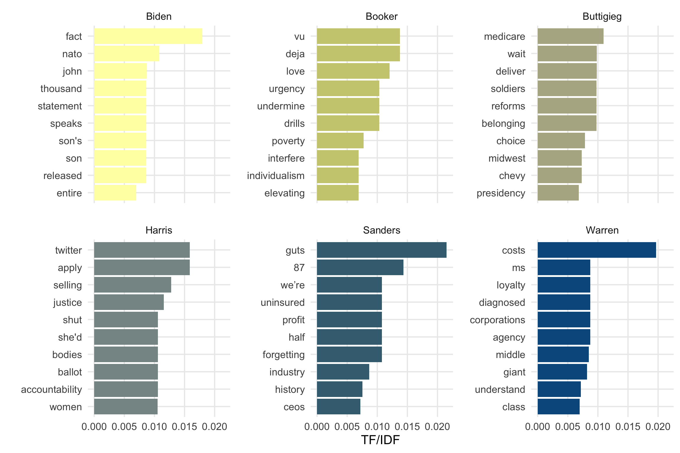

wrap-up

Okay, I think that was a fairly quick overview of some of tidytext’s capabilities, but there’s so much more beyond what I’ve covered here! I really recommend looking at Julia & Dave’s book, and I’d like to explore some other analysis methods (such as topic modeling, which tidytext supports) in future posts. Please feel free to let me know if you’ve found this useful, or if there’s something I can better explain. Happy text mining!